Skip to main content
Exclude a path from WSS 3.0 on Windows Server 2008
Recursive CTEs continued ...
In this post, I will finish the discussion of recursive CTEs that I began in my last post. I will continue to use the CTE examples from Books Online. To run these examples, you'll need to install the Adventure Works Cycles OLTP sample database.
In my last post, I explained that all recursive queries follow the same pattern of one or more anchor sub-selects and one or more recursive sub-selects combined by a UNION ALL. Similarly, all recursive query plans also follow the same pattern which looks like so:
|--Index Spool(WITH STACK)
|--Concatenation
|--Compute Scalar(DEFINE:([Expr10XX]=(0)))
| |-- ... anchor sub-select plan(s) ...
|--Assert(WHERE:(CASE WHEN [Expr10ZZ]>(100) THEN (0) ELSE NULL END))
|--Nested Loops(Inner Join, OUTER REFERENCES:([Expr10YY], [Recr10XX], ...))
|--Compute Scalar(DEFINE:([Expr10ZZ]=[Expr10YY]+(1)))
| |--Table Spool(WITH STACK)
|-- ... recursive sub-select plan(s) ...
Because of this basic plan shape, SQL Server cannot execute recursive queries using parallel plans. There are two basic problems. First, the stack spool does not support parallel execution. Second, the nested loops join does not support parallel execution on its inner input.
Finally, let's look at how the placement of a WHERE clause can have a big impact on the performance of a recursive query. In my last post, I dissected a recursive query that returns a list of all employees and their level within the organization. Suppose that we want to run the same query but limit the results to those employees in the first two levels. We could write the following query (which you'll also find in Books Online) with an extra WHERE clause to limit the results:
WITH DirectReports(ManagerID, EmployeeID, EmployeeLevel) AS
(
SELECT ManagerID, EmployeeID, 0 AS EmployeeLevel
FROM HumanResources.Employee
WHERE ManagerID IS NULL
UNION ALL
SELECT e.ManagerID, e.EmployeeID, EmployeeLevel + 1
FROM HumanResources.Employee e
INNER JOIN DirectReports d
ON e.ManagerID = d.EmployeeID
)
SELECT ManagerID, EmployeeID, EmployeeLevel
FROM DirectReports
WHERE EmployeeLevel <= 2
This query computes uses essentially the same plan as the query without the extra WHERE clause. The WHERE clause simply introduces a filter operator at the root of the plan:
Rows Executes 34 1 |--Filter(WHERE:([Recr1012]<=(2))) 290 1 |--Index Spool(WITH STACK) 290 1 |--Concatenation 0 0 |--Compute Scalar(DEFINE:([Expr1013]=(0))) 0 0 | |--Compute Scalar(DEFINE:([Expr1003]=(0))) 1 1 | |--Index Seek(OBJECT:([Employee].[IX_Employee_ManagerID]), SEEK:([ManagerID]=NULL) ...) 289 1 |--Assert(WHERE:(CASE WHEN [Expr1015]>(100) THEN (0) ELSE NULL END)) 289 1 |--Nested Loops(Inner Join, OUTER REFERENCES:([Expr1015], [Recr1006], [Recr1007], [Recr1008])) 0 0 |--Compute Scalar(DEFINE:([Expr1015]=[Expr1014]+(1))) 290 1 | |--Table Spool(WITH STACK) 0 0 |--Compute Scalar(DEFINE:([Expr1009]=[Recr1008]+(1))) 289 290 |--Index Seek(OBJECT:([Employee].[IX_Employee_ManagerID]), SEEK:([ManagerID]=[Recr1007]) ...)
As you can see from the row counts, this query computes the level of every employee in the organization before discarding the results that we do not want. Now, suppose that we instead move the WHERE clause into the recursive sub-select:
WITH DirectReports(ManagerID, EmployeeID, EmployeeLevel) AS
(
SELECT ManagerID, EmployeeID, 0 AS EmployeeLevel
FROM HumanResources.Employee
WHERE ManagerID IS NULL
UNION ALL
SELECT e.ManagerID, e.EmployeeID, EmployeeLevel + 1
FROM HumanResources.Employee e
INNER JOIN DirectReports d
ON e.ManagerID = d.EmployeeID
WHERE EmployeeLevel < 2
)
SELECT ManagerID, EmployeeID, EmployeeLevel
FROM DirectReports
This query is semantically identical to the previous query, but if we look at the plan, we can see that the filter moves into the recursive portion of the plan:
Rows Executes 34 1 |--Index Spool(WITH STACK) 34 1 |--Concatenation 0 0 |--Compute Scalar(DEFINE:([Expr1013]=(0))) 0 0 | |--Compute Scalar(DEFINE:([Expr1003]=(0))) 1 1 | |--Index Seek(OBJECT:([Employee].[IX_Employee_ManagerID]), SEEK:([ManagerID]=NULL) ...) 33 1 |--Assert(WHERE:(CASE WHEN [Expr1015]>(100) THEN (0) ELSE NULL END)) 33 1 |--Nested Loops(Inner Join, OUTER REFERENCES:([Expr1015], [Recr1006], [Recr1007], [Recr1008])) 0 0 |--Compute Scalar(DEFINE:([Expr1015]=[Expr1014]+(1))) 34 1 | |--Table Spool(WITH STACK) 0 0 |--Compute Scalar(DEFINE:([Expr1009]=[Recr1008]+(1))) 33 34 |--Nested Loops(Inner Join) 7 34 |--Filter(WHERE:(STARTUP EXPR([Recr1008]<(2)))) 7 7 | |--Constant Scan 33 7 |--Index Seek(OBJECT:([Employee].[IX_Employee_ManagerID]), SEEK:([ManagerID]=[Recr1007]) ...)
Notice from the row counts that the new plan computes only the portion of the result set that really interests us and then terminates the recursion.
You may also observe than the plan now has a startup filter. An ordinary filter reads rows from its input tree and then evaluates a Boolean expression on each row to determine whether to return it. A startup filter evaluates its expression only once per execution. The expression does not depend on the input rows. If the expression evaluates to true, the startup filter returns all of its input rows. If the expression evaluates to false, the startup filter returns no rows.
In this example, if the startup filter expression evaluates to true, the constant scan returns one row to the nested loops join immediately above the filter and this join then executes the index seek on its inner input. However, if the startup filter expression evaluates to false, the filter and then the nested loops join return no rows.
While there are many scenarios where a startup filter is genuinely useful, this plan is slightly more complex than is really necessary. The plan could have used an ordinary filter:
|--Index Spool(WITH STACK)
|--Concatenation
|--Compute Scalar(DEFINE:([Expr1013]=(0)))
| |--Compute Scalar(DEFINE:([Expr1003]=(0)))
| |--Index Seek(OBJECT:([HumanResources].[Employee].[IX_Employee_ManagerID]), SEEK:([HumanResources].[Employee].[ManagerID]=NULL) ORDERED FORWARD)
|--Assert(WHERE:(CASE WHEN [Expr1015]>(100) THEN (0) ELSE NULL END))
|--Nested Loops(Inner Join, OUTER REFERENCES:([Expr1015], [Recr1006], [Recr1007], [Recr1008]))
|--Filter(WHERE:([Recr1008]<(2)))
| |--Compute Scalar(DEFINE:([Expr1015]=[Expr1014]+(1)))
| |--Table Spool(WITH STACK)
|--Compute Scalar(DEFINE:([Expr1009]=[Recr1008]+(1)))
|--Index Seek(OBJECT:([HumanResources].[Employee].[IX_Employee_ManagerID] AS [e]), SEEK:([e].[ManagerID]=[Recr1007]) ORDERED FORWARD)
Note that this plan is artificial. You cannot get SQL Server to generate it.
Repeatable Read Isolation Level
In my last two posts, I showed how queries running at read committed isolation level may generate unexpected results in the presence of concurrent updates. Many but not all of these results can be avoided by running at repeatable read isolation level. In this post, I'll explore how concurrent updates may affect queries running at repeatable read.
Unlike a read committed scan, a repeatable read scan retains locks on every row it touches until the end of the transaction. Even rows that do not qualify for the query result remain locked. These locks ensure that the rows touched by the query cannot be updated or deleted by a concurrent session until the current transaction completes (whether it is committed or rolled back). These locks do not protect rows that have not yet been scanned from updates or deletes and do not prevent the insertion of new rows amid the rows that are already locked. The following graphic illustrates this point:
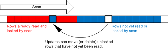
Note that the capability to insert new "phantom" rows between locked rows that have already been scanned is the principle difference between the repeatable read and serializable isolation levels. A serializable scan acquires a key range lock which prevents the insertion of any new rows anywhere within the range (as well as the update or deletion of any existing rows within the range).
In the remainder of this post, I'll give a couple of examples of how we can get unexpected results even while running queries at repeatable read isolation level. These examples are similar to the ones from my previous two posts.
Row Movement
First, let's see how we can move a row and cause a repeatable read scan to miss it. As with all of the other example in this series of posts, we'll need two sessions. Begin by creating this simple table:
create table t (a int primary key, b int)
insert t values (1, 1)
insert t values (2, 2)
insert t values (3, 3)
Next, in session 1 lock the second row:
begin tran
update t set b = 2 where a = 2
Now, in session 2 run a repeatable read scan of the table:
select * from t with (repeatableread)
This scan reads the first row then blocks waiting for session 1 to release the lock it holds on the second row. While the scan is blocked, in session 1 let's move the third row to the beginning of the table before committing the transaction and releasing the exclusive lock blocking session 2:
update t set a = 0 where a = 3
commit tran
As we expect, session 2 completely misses the third row and returns just two rows:
a b c ----------- ----------- ----------- 1 1 1 2 2 2
Note that if we change the experiment so that session 1 tries to touch the first row in the table, it will cause a deadlock with session 2 which holds a lock on this row.
Phantom Rows
Let's also take a look at how phantom rows can cause unexpected results. This experiment is similar to the nested loops join experiment from my previous post. Begin by creating two tables:
create table t1 (a1 int primary key, b1 int)
insert t1 values (1, 9)
insert t1 values (2, 9)
create table t2 (a2 int primary key, b2 int)
Now, in session 1 lock the second row of table t1:
begin tran
update t1 set a1 = 2 where a1 = 2
Next, in session 2 run the following outer join at repeatable read isolation level:
set transaction isolation level repeatable read
select * from t1 left outer join t2 on b1 = a2
The query plan for this join uses a nested loops join:
|--Nested Loops(Left Outer Join, WHERE:([t1].[b1]=[t2].[a2]))
|--Clustered Index Scan(OBJECT:([t1].[PK__t1]))
|--Clustered Index Scan(OBJECT:([t2].[PK__t2]))
This plan scans the first row from t1, tries to join it with t2, finds there are no matching rows, and outputs a null extended row. It then blocks waiting for session 1 to release the lock on the second row of t1. Finally, in session 1, insert a new row into t2 and release the lock:
insert t2 values (9, 0)
commit tran
Here is the output from the outer join:
a1 b1 a2 b2 ----------- ----------- ----------- ----------- 1 9 NULL NULL 2 9 9 0
Notice that we have both a null extended and a joined row for the same join key!
Summary
As I pointed out at the conclusion of my previous post, I want to emphasize that the above results are not incorrect but rather are a side effect of running at a reduced isolation level. SQL Server guarantees that the committed data is consistent at all times.
CLARIFICATION 8/26/2008: The above examples work as I originally described if they are executed in tempdb. However, the SELECT statements in session 2 may not block as described if the examples are executed in other databases due to an optimization where SQL Server avoids acquiring read committed locks when it knows that no data has changed on a page. If you encounter this problem, either run these examples in tempdb or change the UPDATE statements in session 1 so that they actually change the data in the updated row. For instance, for the first example try "update t set b = 12 where a = 2".
ROWCOUNT Top
If you've looked at any insert, update, or delete plans, including those used in some of my posts, you've probably noticed that nearly all such plans include a top operator. For example, the following update statement yields the following plan:
CREATE TABLE T (A INT)
INSERT T VALUES (0)
INSERT T VALUES (1)
INSERT T VALUES (2)
UPDATE T SET A = A + 1
Rows Executes
3 1 UPDATE [T] set [A] = [A]+@1
3 1 |--Table Update(OBJECT:([T]), SET:([T].[A] = [Expr1004]))
0 0 |--Compute Scalar(DEFINE:([Expr1004]=[T].[A]+[@1]))
3 1 |--Top(ROWCOUNT est 0)
3 1 |--Table Scan(OBJECT:([T]))
What is that top operator doing right above the table scan?
It is a ROWCOUNT top. It is used to implement SET ROWCOUNT functionality. The "est 0" indicates that SET ROWCOUNT was 0 when the query was compiled. (I suppose "est" is short for "estimate" though the value at compilation time has no impact on query optimization or execution.) Recall that a value of 0 means return or update all rows. Since SET ROWCOUNT was 0 at execution time as well, we can see from the STATISTICS PROFILE output that all 3 rows were updated.
Now try the following:
SET ROWCOUNT 1
UPDATE T SET A = A + 1
Rows Executes
1 1 UPDATE [T] set [A] = [A]+@1
1 1 |--Table Update(OBJECT:([T]), SET:([T].[A] = [Expr1004]))
0 0 |--Compute Scalar(DEFINE:([Expr1004]=[T].[A]+[@1]))
1 1 |--Top(ROWCOUNT est 0)
1 1 |--Table Scan(OBJECT:([T]))
Although we get the same plan including the ROWCOUNT top with the same "estimate," this time SET ROWCOUNT was 1 at execution time, the top returned only one row from the table scan, and we can see that only 1 row was updated.
If we force a recompile, we see that the value of the "estimate" changes:
SET ROWCOUNT 1
UPDATE T SET A = A + 1 OPTION (RECOMPILE)
Rows Executes
1 1 UPDATE T SET A = A + 1 OPTION (RECOMPILE)
1 1 |--Table Update(OBJECT:([T]), SET:([T].[A] = [Expr1004]))
0 0 |--Compute Scalar(DEFINE:([Expr1004]=[T].[A]+(1)))
1 1 |--Top(ROWCOUNT est 1)
1 1 |--Table Scan(OBJECT:([T]))
Why doesn't SQL Server add a ROWCOUNT top to select statements?
For example, the following query plan does not include a top yet only returns 1 row:
SET ROWCOUNT 1
SELECT * FROM T
Rows Executes
1 1 SELECT * FROM T
1 1 |--Table Scan(OBJECT:([T]))
SQL Server implements SET ROWCOUNT for select statements by simply counting and returning the correct number of rows from the root of the plan. Although this strategy might work for a really trivial update plan such as the one above, it would not work for more complex update plans. For instance, if we add a unique index to our table, the update plan becomes substantially more complex:
CREATE UNIQUE INDEX TA ON T(A)
UPDATE T SET A = A + 1
Rows Executes
2 1 UPDATE [T] set [A] = [A]+@1
2 1 |--Index Update(OBJECT:([T].[TA]), SET:([Bmk10061024] = [Bmk1006],[A1025] = [T].[A]))
2 1 |--Collapse(GROUP BY:([T].[A]))
2 1 |--Filter(WHERE:(NOT [Expr1021]))
2 1 |--Sort(ORDER BY:([T].[A] ASC, [Act1023] ASC))
2 1 |--Split
1 1 |--Table Update(OBJECT:([T]), SET:([T].[A] = [Expr1004]))
1 1 |--Compute Scalar(DEFINE:([Expr1021]=[Expr1021]))
0 0 |--Compute Scalar(DEFINE:([Expr1021]=CASE WHEN [Expr1005] THEN (1) ELSE (0) END))
0 0 |--Compute Scalar(DEFINE:([Expr1004]=[T].[A]+(1), [Expr1005]=CASE WHEN [T].[A] = ([T].[A]+(1)) THEN (1) ELSE (0) END))
1 1 |--Top(ROWCOUNT est 1)
1 1 |--Table Scan(OBJECT:([T]))
I'm not going to try in this post to explain all of the details of the above plan. I'll save that for a future post. However, observe that in updating 1 row, the root of this plan returns 2 rows. Counting 1 row from the root of this plan would not achieve an accurate result. By placing the ROWCOUNT top above the table scan, the optimizer can ensure that the server updates exactly the correct number of rows regardless of the complexity of the remainder of the plan.
Semi-join Transformation
In several of my prior posts, I've given examples of semi-joins. Recall that semi-joins essentially return a row from one input if we can find at least one matching row from the other input. Here is a simple example:
create table T1 (a int, b int)
create table T2 (a int, b int)
set nocount on
declare @i int
set @i = 0
while @i < 10000
begin
insert T1 values(@i, @i)
set @i = @i + 1
end
set nocount on
declare @i int
set @i = 0
while @i < 100
begin
insert T2 values(@i, @i)
set @i = @i + 1
end
select * from T1
where exists (select * from T2 where T2.a = T1.a)
| Rows | Executes | |
| 100 | 1 | |--Hash Match(Right Semi Join, HASH:([T2].[a])=([T1].[a]), RESIDUAL:([T2].[a]=[T1].[a])) |
| 100 | 1 | |--Table Scan(OBJECT:([T2])) |
| 10000 | 1 | |--Table Scan(OBJECT:([T1])) |
Note that the optimizer chooses a hash join and correctly builds a hash table on the smaller input T2 which has only 100 rows and probes with the larger input T1 which has 10,000 rows.
Transformation
Now, let's suppose we want to create an index to speed up this query. Perhaps we'd like to get a plan with an index nested loops join. Should we create an index on T1 or T2? Keep in mind that nested loops join only supports left semi-join not right semi-join. If we get a nested loops semi-join plan, T1 will be the outer table and T2 will be the inner table. Thus, we might be tempted to create an index on T2:
create clustered index T2a on T2(a)
Unfortunately, this index does not change the plan. The optimizer has decided that 10,000 index lookups (one for each row of T1) is still more expensive than the hash join. Fortunately, we have another less obvious option. We can create an index on the larger T1 table:
create clustered index T1a on T1(a)
select * from T1
where exists (select * from T2 where T2.a = T1.a)
Now we get an index nested loops join:
| Rows | Executes | |
| 100 | 1 | |--Nested Loops(Inner Join, OUTER REFERENCES:([T2].[a], [Expr1009]) WITH UNORDERED PREFETCH) |
| 100 | 1 | |--Stream Aggregate(GROUP BY:([T2].[a])) |
| 100 | 1 | | |--Clustered Index Scan(OBJECT:([T2].[T2a]), ORDERED FORWARD) |
| 100 | 100 | |--Clustered Index Seek(OBJECT:([T1].[T1a]), SEEK:([T1].[a]=[T2].[a]) ORDERED FORWARD) |
But wait a minute! This plan has an inner join. What happened to the semi-join? Remember that the semi-join simply returns each row of T1 that matches at least one row of T2. We can use an inner join to find these matches so long as we do not return any row of T1 more than once. In this plan, we use the ordered clustered index scan of T2 and the stream aggregate to eliminate any duplicates values of T2.a. Then, when we join these T2 rows with T1, we know that we can match each T1 row exactly once. Note that unlike the original hash join plan which touched all 10,000 rows of T1, this plan performs only 100 distinct index lookups on T1.
When is this transformation a good idea?
Transforming the semi-join to an inner join helps when, as in this example, we have a large number of rows on the "preserved" side of the join (T1 in this example) and the transformation enables an index seek that would have otherwise been impossible.
The transformation also makes sense if the number of rows on the "lookup" side of the join is very large but most of the rows are duplicates. Since the semi-join does not depend on the duplicates, we can eliminate them. For example, let's drop the index on T1 and create a new 10,000 row table T3 that is all duplicates:
drop index T1.T1a
create table T3 (a int, b int)
set nocount on
declare @i int
set @i = 0
while @i < 10000
begin
insert T3 values(0, @i)
set @i = @i + 1
end
select * from T1
where exists (select * from T3 where T3.a = T1.a)
| Rows | Executes | |
| 1 | 1 | |--Hash Match(Inner Join, HASH:([T3].[a])=([T1].[a]), RESIDUAL:([T3].[a]=[T1].[a])) |
| 1 | 1 | |--Hash Match(Aggregate, HASH:([T3].[a]), RESIDUAL:([T3].[a] = [T3].[a])) |
| 10000 | 1 | | |--Table Scan(OBJECT:([T3])) |
| 10000 | 1 | |--Table Scan(OBJECT:([T1])) |
Notice that even though we have no indexes and use the hash join plan, we still transform the semi-join into an inner join. This time, since we do not have an index, we use a hash aggregate to eliminate duplicate values of T3.a. Without the transformation, the hash join would have built a hash table on all 10,000 rows in T3. With the transformation, it builds a hash table on a single row.
Unique index
If we add a unique index so that duplicate values of T2.a are not possible, the optimizer no longer needs to eliminate duplicates and can always perform this transformation for free. For example:
create unique clustered index T2a on T2(a) with (drop_existing = on)
select * from T1
where exists (select * from T2 where T2.a = T1.a)
| Rows | Executes | |
| 100 | 1 | |--Hash Match(Inner Join, HASH:([T2].[a])=([T1].[a]), RESIDUAL:([T2].[a]=[T1].[a])) |
| 100 | 1 | |--Clustered Index Scan(OBJECT:([T2].[T2a])) |
| 10000 | 1 | |--Table Scan(OBJECT:([T1])) |
Since we dropped the index on T1 (see above), we get the hash join plan again. However, unlike the original right semi-join plan, now we get an inner join. There is no need for a semi-join because the optimizer knows that there can be no duplicates in T2 and that the semi-join and inner join plans are equivalent.
Stay tuned …
This post will probably be my last of the year, but I will be back in January to continue writing about parallelism, partitioned tables, and other query processing topics.
Sequential Read Ahead
Balancing CPU and I/O throughput is essential to achieve good overall performance and to maximize hardware utilization. SQL Server includes two asynchronous I/O mechanisms - sequential read ahead and random prefetching - that are designed to address this challenge.
To understand why asynchronous I/O is so important, consider the CPU to I/O performance gap. The memory subsystem on a modern CPU can deliver data sequentially at roughly 5 Gbytes per second per socket (or for non-NUMA machines for all sockets sharing the same bus) and (depending on how you measure it) can fetch random memory locations at roughly 10 to 50 million accesses per second. By comparison, a high end 15K SAS hard drive can read only 125 Mbytes per second sequentially and can perform only 200 random I/Os per second (IOPS). Solid State Disks (SSDS) can reduce the gap between sequential and random I/O performance by eliminating the moving parts from the equation, but a performance gap remains. In an effort to close this performance gap, it is not uncommon for servers to have a ratio of 10 or more drives for every CPU. (It is also important to consider and balance the entire I/O subsystem including the number and type of disk controllers not just the drives themselves but that is not the focus of this post.)
Unfortunately, a single CPU issuing only synchronous I/Os can keep only one spindle active at a time. For a single CPU to exploit the available bandwidth and IOPs of multiple spindles effectively the server must issue multiple I/Os asynchronously. Thus, SQL Server includes the aforementioned read ahead and prefetching mechanisms. In this post, I'll take a look at sequential read ahead.
When SQL Server performs a sequential scan of a large table, the storage engine initiates the read ahead mechanism to ensure that pages are in memory and ready to scan before they are needed by the query processor. The read ahead mechanism tries to stay 500 pages ahead of the scan. We can see the read ahead mechanism in action by checking the output of SET STATISTICS IO ON. For example, I ran the following query on a 1GB scale factor TPC-H database. The LINEITEM table has roughly 6 million rows.
SET STATISTICS IO ON
SELECT COUNT(*) FROM LINEITEM
Table 'LINEITEM'. Scan count 3, logical reads 22328, physical reads 3, read-ahead reads 20331, lob logical reads 0, lob physical reads 0, lob read-ahead reads 0.
Repeating the query a second time shows that the table is now cached in the buffer pool:
SELECT COUNT(*) FROM LINEITEM
Table 'LINEITEM'. Scan count 3, logical reads 22328, physical reads 0, read-ahead reads 0, lob logical reads 0, lob physical reads 0, lob read-ahead reads 0.
For sequential I/O performance, it is important to distinguish between allocation ordered and index ordered scans. An allocation ordered scan tries to read pages in the order in which they are physically stored on disk while an index ordered scan reads pages according to the order in which the data on those index pages is sorted. (Note that in many cases there are multiple levels of indirection such as RAID devices or SANS between the logical volumes that SQL Server sees and the physical disks. Thus, even an allocation ordered scan may in fact not be truly optimally ordered.) Although SQL Server tries to sort and read pages in allocation order even for an index ordered scan, an allocation ordered scan is generally going to be faster since pages are read in the order that they are written on disk with the minimal number of seeks. Heaps have no inherent order and, thus, are always scanned in allocation order. Indexes are scanned in allocation order only if the isolation level is read uncommitted (or the NOLOCK hint is used) and only if the query process does not request an ordered scan. Defragmenting indexes can help to ensure that index ordered scans perform on par with allocation ordered scans.
In my next post, I'll take a look at random prefetching.
Serializable vs. Snapshot Isolation Level
Both the serializable and snapshot isolation levels provide a read consistent view of the database to all transactions. In either of these isolation levels, a transaction can only read data that has been committed. Moreover, a transaction can read the same data multiple times without ever observing any concurrent transactions making changes to this data. The unexpected read committed and repeatable read results that I demonstrated in my prior few posts are not possible in serializable or snapshot isolation level.
Notice that I used the phrase "without ever observingany ... changes." This choice of words is deliberate. In serializable isolation level, SQL Server acquires key range locks and holds them until the end of the transaction. A key range lock ensures that, once a transaction reads data, no other transaction can alter that data - not even to insert phantom rows - until the transaction holding the lock completes. In snapshot isolation level, SQL Server does not acquire any locks. Thus, it is possible for a concurrent transaction to modify data that a second transaction has already read. The second transaction simply does not observe the changes and continues to read an old copy of the data.
Serializable isolation level relies on pessimistic concurrency control. It guarantees consistency by assuming that two transactions might try to update the same data and uses locks to ensure that they do not but at a cost of reduced concurrency - one transaction must wait for the other to complete and two transactions can deadlock. Snapshot isolation level relies on optimistic concurrency control. It allows transactions to proceed without locks and with maximum concurrency, but may need to fail and rollback a transaction if two transactions attempt to modify the same data at the same time.
It is clear there are differences in the level of concurrency that can be achieved and in the failures (deadlocks vs. update conflicts) that are possible with the serializable and snapshot isolation levels.
How about transaction isolation? How do serializable and snapshot differ in terms of the transaction isolation that they confer? It is simple to understand serializable. For the outcome of two transactions to be considered serializable, it must be possible to achieve this outcome by running one transaction at a time in some order.
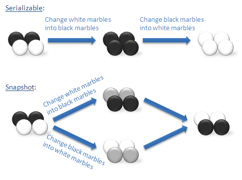
Snapshot does not guarantee this level of isolation. A few years ago, Jim Gray shared with me the following excellent example of the difference. Imagine that we have a bag containing a mixture of white and black marbles. Suppose that we want to run two transactions. One transaction turns each of the white marbles into black marbles. The second transaction turns each of the black marbles into white marbles. If we run these transactions under serializable isolation, we must run them one at a time. The first transaction will leave a bag with marbles of only one color. After that, the second transaction will change all of these marbles to the other color. There are only two possible outcomes: a bag with only white marbles or a bag with only black marbles.
If we run these transactions under snapshot isolation, there is a third outcome that is not possible under serializable isolation. Each transaction can simultaneously take a snapshot of the bag of marbles as it exists before we make any changes. Now one transaction finds the white marbles and turns them into black marbles. At the same time, the other transactions finds the black marbles - but only those marbles that where black when we took the snapshot - not those marbles that the first transaction changed to black - and turns them into white marbles. In the end, we still have a mixed bag of marbles with some white and some black. In fact, we have precisely switched each marble.
The following graphic illustrates the difference:
We can demonstrate this outcome using SQL Server. Note that snapshot isolation is only available in SQL Server 2005 and must be explicitly enabled on your database:
alter database database_name set allow_snapshot_isolation on
Begin by creating a simple table with two rows representing two marbles:
create table marbles (id int primary key, color char(5))
insert marbles values(1, 'Black')
insert marbles values(2, 'White')
Next, in session 1 begin a snaphot transaction:
set transaction isolation level snapshot
begin tran
update marbles set color = 'White' where color = 'Black'
Now, before committing the changes, run the following in session 2:
set transaction isolation level snapshot
begin tran
update marbles set color = 'Black' where color = 'White'
commit tran
Finally, commit the transaction in session 1 and check the data in the table:
commit tran
select * from marbles
Here are the results:
id color ----------- ----- 1 White 2 Black
As you can see marble 1 which started out black is now white and marble 2 which started out white is now black. If you try this same experiment with serializable isolation, one transaction will wait for the other to complete and, depending on the order, both marbles will end up either white or black.
Subqueries in BETWEEN and CASE Statements
Consider the following query:
CREATE TABLE T1 (A INT, B1 INT, B2 INT)
CREATE TABLE T2 (A INT, B INT)
SELECT *
FROM T1
WHERE (SELECT SUM(T2.B) FROM T2 WHERE T2.A = T1.A) BETWEEN T1.B1 AND T1.B2
Observe that the subquery in this query only needs to be evaluated once for each row of T1. Indeed running on SQL Server 2000, we get the following plan (with the portion of the plan corresponding to the subquery in bold):
|--Nested Loops(Inner Join, OUTER REFERENCES:([T2].[A], [Expr1004]))
** |--Compute Scalar(DEFINE:([Expr1004]=If ([Expr1014]=0) then NULL else [Expr1015]))
| |--Stream Aggregate(GROUP BY:([T2].[A]) DEFINE:([Expr1014]=COUNT_BIG([T2].[B]), [Expr1015]=SUM([T2].[B])))
| |--Sort(ORDER BY:([T2].[A] ASC))
| |--Table Scan(OBJECT:([T2]))
** |--Filter(WHERE:([Expr1004]<=[T1].[B2]))
|--Index Spool(SEEK:([T1].[A]=[T2].[A] AND [T1].[B1] <= [Expr1004]))
|--Table Scan(OBJECT:([T1]))
Now let's look at the query plan we get (with SQL Server 2005 or SQL Server 2008):
|--Nested Loops(Inner Join, OUTER REFERENCES:([T2].[A], [Expr1008], [Expr1014]))
|--Merge Join(Inner Join, MERGE:([T2].[A])=([T2].[A]), RESIDUAL:([T2].[A]=[T2].[A]))
** | |--Compute Scalar(DEFINE:([Expr1008]=CASE WHEN [Expr1026]=(0) THEN NULL ELSE [Expr1027] END))
| | |--Stream Aggregate(GROUP BY:([T2].[A]) DEFINE:([Expr1026]=COUNT_BIG([T2].[B]), [Expr1027]=SUM([T2].[B])))
| | |--Sort(ORDER BY:([T2].[A] ASC))
| | |--Table Scan(OBJECT:([T2]))
| |--Compute Scalar(DEFINE:([Expr1014]=CASE WHEN [Expr1028]=(0) THEN NULL ELSE [Expr1029] END))
| |--Stream Aggregate(GROUP BY:([T2].[A]) DEFINE:([Expr1028]=COUNT_BIG([T2].[B]), [Expr1029]=SUM([T2].[B])))
| |--Sort(ORDER BY:([T2].[A] ASC))
| |--Table Scan(OBJECT:([T2]))
** |--Filter(WHERE:([Expr1014]<=[T1].[B2]))
|--Index Spool(SEEK:([T1].[A]=[T2].[A] AND [T1].[B1] <= [Expr1008]))
|--Table Scan(OBJECT:([T1]))
Notice that the subquery is actually evaluated twice. There are two scans of T2, two sorts, and two stream aggregates. I've highlighted both sets of operators in bold.
Why is SQL Server evaluating the subquery twice? The answer is that SQL Server transforms "X BETWEEEN Y AND Z" into "X <= Y AND X >= Z". If as in this query, X is a subquery, the subquery is repeated:
SELECT *
FROM T1
WHERE (SELECT SUM(T2.B) FROM T2 WHERE T2.A = T1.A) >= T1.B1 AND
(SELECT SUM(T2.B) FROM T2 WHERE T2.A = T1.A) <= T1.B2
This transformation occurs very early in the processing of the query. Unfortunately, after that point, SQL Server 2005 and SQL Server 2008 do not realize that the subquery is a common subexpression and they evaluate it as if there were two completely different subqueries.
You may also have noticed that, instead of scanning T1 first and then evaluating the subquery for each row of T1, this plan actually scans T2 first. This join order results from the optimizer decorrelating the subqueries.
So, how can we get SQL Server to evaluate the subquery only once? There are actually multiple solutions and all involve rewriting the query to calculate the subquery separately from the BETWEEN clause so that when SQL Server transforms the BETWEEN clause, it does not also duplicate the subquery. Here are some examples:
SELECT Q.A, Q.B1, Q.B2
FROM
(
SELECT *, (SELECT SUM(T2.B) FROM T2 WHERE T2.A = T1.A) SUM_B
FROM T1
) Q
WHERE SUM_B BETWEEN Q.B1 AND Q.B2
SELECT T1.*
FROM T1 CROSS APPLY (SELECT SUM(T2.B) SUM_B FROM T2 WHERE T2.A = T1.A) Q
WHERE Q.SUM_B BETWEEN T1.B1 AND T1.B2
SELECT T1.*
FROM T1, (SELECT T2.A, SUM(T2.B) SUM_B FROM T2 GROUP BY T2.A) Q
WHERE T1.A = Q.A AND Q.SUM_B BETWEEN T1.B1 AND T1.B2
All three of these rewrites produce the same plan:
|--Nested Loops(Inner Join, OUTER REFERENCES:([T2].[A], [Expr1008]))
** |--Compute Scalar(DEFINE:([Expr1008]=CASE WHEN [Expr1016]=(0) THEN NULL ELSE [Expr1017] END))
| |--Stream Aggregate(GROUP BY:([T2].[A]) DEFINE:([Expr1016]=COUNT_BIG([T2].[B]), [Expr1017]=SUM([T2].[B])))
| |--Sort(ORDER BY:([T2].[A] ASC))
| |--Table Scan(OBJECT:([T2]))
** |--Filter(WHERE:([Expr1008]<=[T1].[B2]))
|--Index Spool(SEEK:([T1].[A]=[T2].[A] AND [T1].[B1] <= [Expr1008]))
|--Table Scan(OBJECT:([T1]))
SQL Server also transforms a CASE statement of the form:
CASE X
WHEN Y1 THEN Z1
WHEN Y2 THEN Z2
...
ELSE ZN
END
Into:
CASE
WHEN X = Y1 THEN Z1
WHEN X = Y2 THEN Z2
...
ELSE ZN
END
Thus, CASE statements can yield the same problematic behavior if X is a subquery. Unfortunately, with a CASE statement, the number of times that the subquery is reevaluated depends on the number WHEN clauses and can be quite large. Here is a simple query that illustrates the problem:
SELECT *,
CASE (SELECT SUM(T2.B) FROM T2 WHERE T2.A = T1.A)
WHEN T1.B1 THEN 'B1'
WHEN T1.B2 THEN 'B2'
ELSE NULL
END CASE_B
FROM T1
Here is the SQL Server 2000 plan:
|--Compute Scalar(DEFINE:([Expr1007]=If ([Expr1004]=[T1].[B1]) then 'B1' else If ([Expr1004]=[T1].[B2]) then 'B2' else NULL))
|--Nested Loops(Left Outer Join, OUTER REFERENCES:([T1].[A]))
|--Table Scan(OBJECT:([T1]))
|--Hash Match(Cache, HASH:([T1].[A]), RESIDUAL:([T1].[A]=[T1].[A]))
** |--Compute Scalar(DEFINE:([Expr1004]=If ([Expr1020]=0) then NULL else [Expr1021]))
|--Stream Aggregate(DEFINE:([Expr1020]=COUNT_BIG([T2].[B]), [Expr1021]=SUM([T2].[B])))
|--Table Scan(OBJECT:([T2]), WHERE:([T2].[A]=[T1].[A]))**
And here is the SQL Server 2005 and SQL Server 2008 plan:
|--Compute Scalar(DEFINE:([Expr1016]=CASE WHEN [Expr1008]=[T1].[B1] THEN 'B1' ELSE CASE WHEN [Expr1014]=[T1].[B2] THEN 'B2' ELSE NULL END END))
|--Nested Loops(Inner Join, PASSTHRU:([Expr1008]=[T1].[B1]), OUTER REFERENCES:([T1].[A]))
|--Nested Loops(Left Outer Join, OUTER REFERENCES:([T1].[A]))
| |--Table Scan(OBJECT:([T1]))
** | |--Compute Scalar(DEFINE:([Expr1008]=CASE WHEN [Expr1030]=(0) THEN NULL ELSE [Expr1031] END))
| |--Stream Aggregate(DEFINE:([Expr1030]=COUNT_BIG([T2].[B]), [Expr1031]=SUM([T2].[B])))
| |--Table Scan(OBJECT:([T2]), WHERE:([T2].[A]=[T1].[A]))
|--Compute Scalar(DEFINE:([Expr1014]=CASE WHEN [Expr1032]=(0) THEN NULL ELSE [Expr1033] END))
|--Stream Aggregate(DEFINE:([Expr1032]=COUNT_BIG([T2].[B]), [Expr1033]=SUM([T2].[B])))
|--Table Scan(OBJECT:([T2]), WHERE:([T2].[A]=[T1].[A]))**
Finally, the same solutions once again apply:
SELECT Q.A, Q.B1, Q.B2,
CASE Q.SUM_B
WHEN Q.B1 THEN 'B1'
WHEN Q.B2 THEN 'B2'
ELSE NULL
END CASE_B
FROM
(
SELECT *, (SELECT SUM(T2.B) FROM T2 WHERE T2.A = T1.A) SUM_B
FROM T1
) Q
SELECT T1.*,
CASE Q.SUM_B
WHEN T1.B1 THEN 'B1'
WHEN T1.B2 THEN 'B2'
ELSE NULL
END CASE_B
FROM T1 CROSS APPLY (SELECT SUM(T2.B) SUM_B FROM T2 WHERE T2.A = T1.A) Q
SELECT T1.*,
CASE Q.SUM_B
WHEN T1.B1 THEN 'B1'
WHEN T1.B2 THEN 'B2'
ELSE NULL
END CASE_B
FROM T1, (SELECT T2.A, SUM(T2.B) SUM_B FROM T2 GROUP BY T2.A) Q
WHERE T1.A = Q.A
The PIVOT Operator
In my next few posts, I'm going to look at how SQL Server implements the PIVOT and UNPIVOT operators. Let's begin with the PIVOT operator. The PIVOT operator takes a normalized table and transforms it into a new table where the columns of the new table are derived from the values in the original table. For example, suppose we want to store annual sales data by employee. We might create a schema such as the following:
CREATE TABLE Sales (EmpId INT, Yr INT, Sales MONEY)
INSERT Sales VALUES(1, 2005, 12000)
INSERT Sales VALUES(1, 2006, 18000)
INSERT Sales VALUES(1, 2007, 25000)
INSERT Sales VALUES(2, 2005, 15000)
INSERT Sales VALUES(2, 2006, 6000)
INSERT Sales VALUES(3, 2006, 20000)
INSERT Sales VALUES(3, 2007, 24000)
Notice that this schema has one row per employee per year. Moreover, notice that in the sample data employees 2 and 3 only have sales data for two of the three years worth of data. Now suppose that we'd like to transform this data into a table that has one row per employee with all three years of sales data in each row. We can achieve this conversion very easily using PIVOT:
SELECT EmpId, [2005], [2006], [2007]
FROM (SELECT EmpId, Yr, Sales FROM Sales) AS s
PIVOT (SUM(Sales) FOR Yr IN ([2005], [2006], [2007])) AS p
I'm not going to delve into the PIVOT syntax which is already documented in Books Online. Suffice it to say that this statement sums up the sales for each employee for each of the specified years and outputs one row per employee. The resulting output is:
EmpId 2005 2006 2007 ----------- --------------------- --------------------- --------------------- 1 12000.00 18000.00 25000.00 2 15000.00 6000.00 NULL 3 NULL 20000.00 24000.00
Notice that SQL Server inserts NULLs for the missing sales data for employees 2 and 3.
The SUM keyword (or some other aggregate) is required. If the Sales table includes multiple rows for a particular employee for a particular year, PIVOT does aggregate them - in this case by summing them - into a single data point in the result. Of course, in this example, since the entry in each "cell" of the output table is the result of summing a single input row, we could just as easily have used another aggregate such as MIN or MAX. I've used SUM since it is more intuitive.
This PIVOT example is reversible. The information in the output table can be used to reconstruct the original input table using an UNPIVOT operation (which I will cover in a later post). However, not all PIVOT operations are reversible. To be reversible, a PIVOT operation must meet the following criteria:
- All of the input data must be transformed. If we include a filter of any kind including on the IN clause, some data may be omitted from the PIVOT result. For example, if we altered the above example only to output sales for 2006 and 2007, clearly we could not reconstruct the 2005 sales data from the result.
- Each cell in the output table must derive from a single input row. If multiple input rows are aggregated into a single cell, there is no way to reconstruct the original input rows.
- The aggregate function must be an identity function (when used on a single input row). SUM, MIN, MAX, and AVG all return the single input value unchanged and, thus, can be reversed. COUNT does not return its input value unchanged and, thus, cannot be reversed.
Here is an example of a non-reversible PIVOT operation. This example, calculates the total sales for all employees for all three years. It does not itemize the output by employee.
SELECT [2005], [2006], [2007]
FROM (SELECT Yr, Sales FROM Sales) AS s
PIVOT (SUM(Sales) FOR Yr IN ([2005], [2006], [2007])) AS p
Here is the output. Each cell represents the sum of two or three rows from the input table.
2005 2006 2007 --------------------- --------------------- --------------------- 27000.00 44000.00 49000.00
In my next post, I'll look at some example PIVOT query plans.
The UNPIVOT Operator
The UNPIVOT operator is the opposite of the PIVOT operator. As I explained in my earlier post, the PIVOT operator takes a normalized table and transforms it into a new table where the columns of the new table are derived from the values in the original table. The UNPIVOT operator takes a pivoted table and transforms it back into a normalized form with one row per data point using the column names as values in the result. For example, suppose we have the following data:
CREATE TABLE PIVOT_Sales(EmpId INT, [2005] MONEY, [2006] MONEY, [2007] MONEY)
INSERT PIVOT_Sales VALUES(1, 12000, 18000, 25000)
INSERT PIVOT_Sales VALUES(2, 15000, 6000, NULL)
INSERT PIVOT_Sales VALUES(3, NULL, 20000, 24000)
This is the output of the PIVOT operation from my earlier posts. There is one row for each employee with up to three years of sales data per row. If there is no sales data for a particular employee for a particular year, we simply insert NULL. We can transform this table back to its original form with a single row per employee per year using the following UNPIVOT statement:
SELECT EmpId, CAST (Yr AS INT) AS Yr, Sales
FROM (SELECT EmpId, [2005], [2006], [2007] FROM PIVOT_Sales) AS p
UNPIVOT (Sales FOR Yr IN ([2005], [2006], [2007])) AS s
I've explicitly casted the Yr column to integer. The default type for the pivot column is NVARCHAR(128). This type is based on the maximum column name length of 128 characters.
The resulting output is:
EmpId Yr Sales ----------- ----------- --------------------- 1 2005 12000.00 1 2006 18000.00 1 2007 25000.00 2 2005 15000.00 2 2006 6000.00 3 2006 20000.00 3 2007 24000.00
Unlike PIVOT operations which may not be reversible, all UNPIVOT operations are reversible (so long as all of the input data is preserved). That is, we can always transform the output of an UNPIVOT operation back into the original table using an appropriate PIVOT operation. Unlike PIVOT operator, the UNPIVOT operator does not require or support aggregation functions.
Let's look at the plan for the above query:
|--Compute Scalar(DEFINE:([Expr1010]=CONVERT(int,[Expr1009],0)))
|--Filter(WHERE:([Expr1008] IS NOT NULL))
|--Nested Loops(Left Outer Join, OUTER REFERENCES:([PIVOT_Sales].[2005], [PIVOT_Sales].[2006], [PIVOT_Sales].[2007]))
|--Compute Scalar(DEFINE:([PIVOT_Sales].[EmpId]=[PIVOT_Sales].[EmpId]))
| |--Table Scan(OBJECT:([PIVOT_Sales]))
|--Constant Scan(VALUES:((N'2005',[PIVOT_Sales].[2005]),(N'2006',[PIVOT_Sales].[2006]),(N'2007',[PIVOT_Sales].[2007])))
This query plan simply takes each row of the input table and joins it with a constant scan that generates three rows - one for each of the three columns listed in the UNPIVOT IN clause - for each input row. The plan then filters out any rows that have NULL data. (Note that [Expr1008] is the Sales column and [Expr1009] is the Yr column.) There are a couple of points worth noting about this query plan. First, the join must be a nested loops join because the constant scan operator uses the correlated parameters from the outer side of the join to generate rows. There is no way to generate these rows without these correlated parameters. Second, the join need not be a left outer join. The constant scan always produces exactly three rows and, thus, the outer rows always join and are never NULL extended. Nevertheless, the outer join is harmless in this context and behaves like an inner join.
Note that we can write the original query as:
SELECT p.EmpId, Yr, Sales
FROM PIVOT_Sales AS p CROSS APPLY
(
SELECT EmpId, 2005 AS Yr, [2005] AS Sales UNION ALL
SELECT EmpId, 2006, [2006] UNION ALL
SELECT EmpId, 2007, [2007]
) AS s
WHERE Sales IS NOT NULL
This query yields a nearly identical query plan. The UNION ALL syntax produces a similar result to the constant scan except that there are now three constant scans and a concatenation operator:
|--Filter(WHERE:([Union1007] IS NOT NULL))
|--Nested Loops(Inner Join, OUTER REFERENCES:([p].[2005], [p].[2006], [p].[2007]))
|--Table Scan(OBJECT:([tempdb].[dbo].[PIVOT_Sales] AS [p]))
|--Concatenation
|--Constant Scan(VALUES:(((2005))))
|--Constant Scan(VALUES:(((2006))))
|--Constant Scan(VALUES:(((2007))))
In this plan, [Union1007] is the Sales column. We can actually see the definition of [Union1007] from the DefinedValues column of the concatenation operator in the SET SHOWPLAN_ALL ON output:
[Union1006] = ([Expr1003], [Expr1004], [Expr1005]), [Union1007] = ([p].[2005], [p].[2006], [p].[2007])
Notice that the values for [Union1007] are actually derived directly from the correlated parameters of the cross apply (from the PIVOT_Sales table) and not from the constant scans. [Union1006] is the Yr column and the values are derived from the constant scans.
We have moved!
Thanks for visiting! This blog has now been migrated to:
https://techcommunity.microsoft.com/t5/SQL-Server/bg-p/SQLServer/label-name/SQLServerQueryProcessing
What is the difference between sys.dm_db_index_usage_stats and sys.dm_db_index_operational_stats?
SQL Server includes two DMVs - sys.dm_db_index_usage_stats and sys.dm_db_index_operational_stats - that are extremely useful for monitoring which indexes are used as well as how and when they are used. Both DMVs report similar statistics on information such as the number of scans, seeks, and updates to different indexes. These DMVs are documented in Books Online (see here and here) and a simple Web search reveals numerous other postings about these DMVs. However, in my own search, I did not find many direct explanations of the difference between these two valuable DMVs. (You will find a short explanation halfway through this post on the Microsoft SQL Server Customer Advisory Team blog.)
The main difference between these DMVs is simple but important:
sys.dm_db_index_usage_stats records how many times the query optimizer uses an index in a plan. This usage information is recorded again each time the plan is executed. (Compiling a plan alone is not sufficient to record an index's usage.) However, and this is the important part, for the purposes of computing the statistics, it does matter how many times the query processor executes the specific operator that references the index. For that matter, it does not matter whether the query processor executes the operator at all. Mere execution of the plan counts as a single usage for each index used by the plan.
sys.dm_db_index_operational_stats records how many times the storage engine executes a specific operation on the index. These statistics do depend on how many times the query processor executes each operator. If an operator is never executed, the storage engine does not perform any operations on the index and the DMV reports that the index was not used. If an operator is executed multiple times, the storage engine performs multiple operations on the index and the DMV reports that the index was used multiple times.
Update (7/29/2009): The following paragraph is incorrect. See this post for more information.
(Another less important difference between these DMVs is that sys.dm_db_index_usage_stats only reports on indexes that have been used at least once since the server was last restarted while sys.dm_db_index_operational_stats reports on all indexes regardless of whether they have been used.)
Let's try an example to see this difference in action. I'll use the following simple schema:
CREATE TABLE T (A INT, B INT, C INT)
CREATE UNIQUE CLUSTERED INDEX TA ON T(A)
CREATE UNIQUE INDEX TB ON T(B)
As expected, immediately after creating this table, the stats are zero (or just non-existent):
SELECT index_id, user_seeks, user_scans, user_lookups, user_updates
FROM sys.dm_db_index_usage_stats
WHERE database_id = DB_ID('tempdb') and object_id = OBJECT_ID('tempdb..t')
ORDER BY index_id
SELECT index_id, range_scan_count, singleton_lookup_count
FROM sys.dm_db_index_operational_stats (DB_ID('tempdb'), OBJECT_ID('tempdb..t'), NULL, NULL)
ORDER BY index_id
index_id user_seeks user_scans user_lookups user_updates ----------- -------------------- -------------------- -------------------- --------------------
index_id range_scan_count singleton_lookup_count ----------- -------------------- ---------------------- 1 0 0 2 0 0
Now suppose that we do a scan of the clustered index:
SELECT * FROM T
|--Clustered Index Scan(OBJECT:([tempdb].[dbo].[T].[TA]))
Repeating the DMV queries, we see that the clustered index shows one scan in both DMVs. SQL Server records the scan even though the table contains no rows and the query returns an empty result:
index_id user_seeks user_scans user_lookups user_updates ----------- -------------------- -------------------- -------------------- -------------------- 1 0 1 0 0
index_id range_scan_count singleton_lookup_count ----------- -------------------- ---------------------- 1 1 0 2 0 0
Next let's try a singleton lookup on the clustered index:
SELECT * FROM T WHERE A = 1
|--Clustered Index Seek(OBJECT:([tempdb].[dbo].[T].[TA]), SEEK:([tempdb].[dbo].[T].[A]=CONVERT_IMPLICIT(int,[@1],0)) ORDERED FORWARD)
Again the table contains no rows and the query returns an empty result. Nevertheless, the DMVs now report one seek and one singleton lookup:
index_id user_seeks user_scans user_lookups user_updates ----------- -------------------- -------------------- -------------------- -------------------- 1 1 1 0 0
index_id range_scan_count singleton_lookup_count ----------- -------------------- ---------------------- 1 1 1 2 0 0
(Keep in mind that the DMV results are cumulative so you need to subtract the previous values from the current values as you run each of these experiments. Thus, we can disregard the scan that was already reported by the previous example.)
Now let's try something a little more interesting. Let's run a bookmark lookup:
SELECT * FROM T WHERE B = 1
|--Nested Loops(Inner Join, OUTER REFERENCES:([tempdb].[dbo].[T].[A]))
|--Index Seek(OBJECT:([tempdb].[dbo].[T].[TB]), SEEK:([tempdb].[dbo].[T].[B]=CONVERT_IMPLICIT(int,[@1],0)) ORDERED FORWARD)
|--Clustered Index Seek(OBJECT:([tempdb].[dbo].[T].[TA]), SEEK:([tempdb].[dbo].[T].[A]=[tempdb].[dbo].[T].[A]) LOOKUP ORDERED FORWARD)
As expected sys.dm_db_index_usage_stats reports a seek on index TB (index id 2) and a bookmark lookup on the clustered index (index id 1). However, sys.dm_db_index_operational_stats reports only the singleton lookup on index TB but does not report any new activity on the clustered index:
index_id user_seeks user_scans user_lookups user_updates ----------- -------------------- -------------------- -------------------- -------------------- 1 1 1 1 0 2 1 0 0 0
index_id range_scan_count singleton_lookup_count ----------- -------------------- ---------------------- 1 1 1 2 0 1
To understand what has happened, recall how a nested loops join works. The server executes the seek (the singleton lookup) on index TB and, as in the previous example, both DMVs are updated even though the seek returns no rows. However, since the seek on index TB returns no rows, the nested loops join does not execute the clustered index seek (i.e., the bookmark lookup). The server updates sys.dm_db_index_usage_stats to indicate that it executed a query plan that includes a bookmark lookup on table T, but does not update sys.dm_db_index_operational_stats since the query did not actually perform any bookmark lookups.
Next, let's insert three rows into the table and run another bookmark lookup experiment. I'm using a hint to force a bookmark lookup plan. Without the hint, the optimizer would simply use a clustered index scan since the query returns all three rows in the table:
INSERT T VALUES (0, 0, 0), (1, 1, 1), (2, 2, 2)
SELECT * FROM T WITH (INDEX (TB))
|--Nested Loops(Inner Join, OUTER REFERENCES:([tempdb].[dbo].[T].[A]))
|--Index Scan(OBJECT:([tempdb].[dbo].[T].[TB]))
|--Clustered Index Seek(OBJECT:([tempdb].[dbo].[T].[TA]), SEEK:([tempdb].[dbo].[T].[A]=[tempdb].[dbo].[T].[A]) LOOKUP ORDERED FORWARD)
This time sys.dm_db_index_usage_stats reports a scan on index TB and a bookmark lookup on the clustered index (plus the updates from the insert statement). But, sys.dm_db_index_operational_stats reports a scan on index TB and three bookmark lookups on the clustered index:
index_id user_seeks user_scans user_lookups user_updates ----------- -------------------- -------------------- -------------------- -------------------- 1 1 1 2 1 2 1 1 0 1
index_id range_scan_count singleton_lookup_count ----------- -------------------- ---------------------- 1 1 4 2 1 1
When the server executes the above query, it runs the clustered index seek three times - once for each row returned by the index scan. We ran the query only once but it performed three bookmark lookups. Thus, as in the prior example, the server updates sys.dm_db_index_usage_stats to indicate that it executed a query plan that includes a bookmark lookup on table T, but unlike the prior example, it updates sys.dm_db_index_operational_stats to indicate that the query performed three actual bookmark lookups.
I've used bookmark lookups in the above examples, but any nested loops join will produce similar results. At this point, it should be clear that the statistics returned by these two DMVs can differ dramatically.
So, what is the important takeaway from all of these examples? Don't expect the data reported by these two DMVs to match. sys.dm_db_index_usage_stats tells us the proportion of query plans that were executed that use various indexes. This information is useful for concluding how many of the executed query plans might be affected if we drop an index but it does not tell us how many actual operations are performed using each index. sys.dm_db_index_operational_stats, on the other hand, tells us how often the indexes are actually used during the execution of plans and, thus, which indexes are directly contributing to server performance. But, even if sys.dm_db_index_operational_stats indicates that an index is not used very often (or perhaps even that an index is never used), do not automatically conclude that you can drop the index. First, be sure that sys.dm_db_index_usage_stats indicates that no queries depend on the index. In some cases, the presence of an index could change a query plan for the better even though the index itself is not used when the plan is executed.
A Fifteenth-Century Dilbert Cartoon
Reading Judith Barker's excellent Agincourt: Henry V and the Battle That Made England, I came across what is, in effect, an early fifteenth-century Dilbert cartoon. Barker, in discussing the strategic logistical planning for the Agincourt campaign, which Henry V of England undertook by invading France in the early 1400's, notes that gunpowder had been invented, and artillery had appeared on the battlefield. Early cannons, she explains, were not only difficult to aim, being very heavy metal things with no mechanical means of orienting them, but also required considerable effort merely to fire. The ammunition had to be loaded in the front, and a complicated, albeit primitive device, was used to get the gunpowder into the cannon. Consequently--and this is the crucial fact--the typical artillery crew usually only managed to fire their weapon once during a battle.
Now there is a record of a particularly efficient gunner, who, in a battle, was able to fire no less than an amazing three shots from his cannon in the course of a fight. Witnessing this feat, his commanders concluded that he could not have accomplished it were he not in league with the devil. So the gunner was sent off an a pilgrimage to cure his soul.
A Windows Communication Foundation JSONP Service
All of the samples I've found that show how to build a JSONP service using the Windows Communication Foundation have the thing hosted in IIS. IIS is literally the last place I want my Windows Communication Foundation services hosted ... especially because I'll only want them in IIS once I've debugged them, and debugging outside of IIS is much more efficient. Here is a console version of such a service:
using System;
using System.Runtime.Serialization;
using System.ServiceModel;
using System.ServiceModel.Description;
using System.ServiceModel.Web;
namespace Server
{
[DataContract]
public class Some
{
[DataMember]
public string What;
[DataMember]
public string Why;
}
[ServiceContract]
[JavascriptCallbackBehavior(UrlParameterName="method")]
class MyService
{
[OperationContract]
[WebGet(ResponseFormat = WebMessageFormat.Json)]
public Some GetSome(string input)
{
return new Some() { What = "A Shotgun", Why = "Needs an Outcome" };
}
}
class Program
{
const string BaseAddress = "https://localhost:8888/MyService/";
const string EndpointAddress = "MyEndpoint";
static void Main(string[] args)
{
using(ServiceHostBase serviceHost = new ServiceHost(typeof(MyService),new Uri[]{new Uri(Program.BaseAddress)}))
{
WebHttpBinding binding = new WebHttpBinding();
binding.CrossDomainScriptAccessEnabled = true;
ServiceEndpoint endpoint = serviceHost.AddServiceEndpoint("Server.MyService", binding, Program.EndpointAddress);
WebHttpBehavior behavior = new WebHttpBehavior();
WebScriptEnablingBehavior scripting = new WebScriptEnablingBehavior();
endpoint.Behaviors.Add(behavior);
endpoint.Behaviors.Add(scripting);
serviceHost.Open();
Console.WriteLine("Press <ENTER> to terminate this program.");
Console.ReadLine();
}
}
}
}
And here is the HTML page that you can open in the current version of any major browser to see the output from the service:
<!DOCTYPE html PUBLIC "-//W3C//DTD XHTML 1.0 Transitional//EN" "https://www.w3.org/TR/xhtml1/DTD/xhtml1-transitional.dtd">
<html xmlns="https://www.w3.org/1999/xhtml" >
<head>
<title>Untitled Page</title>
<script src="https://ajax.aspnetcdn.com/ajax/jQuery/jquery-1.5.1.js" type="text/javascript"></script>
<script type="text/javascript">
function callback(data) {
alert("Like a " + data.What + " " + data.Why);
}
$(document).ready(
function () {
$("<p>Hello, I am Dynamic Text!</p>").appendTo("body");
$("<p>Attempt</p>").appendTo("body");
$.getJSON("https://localhost:8888/MyService/MyEndpoint/GetSome?method=?", callback);
$("<p>Done</p>").appendTo("body");
}
);
</script>
</head>
<body>
</body>
</html>
Body of Lies
I read a lot of spy fiction. I have observed that the sociology of an espionage organization, as depicted, especially by Len Deighton, is very similar to that of a software development enterprise. While I may expand on that observation in more detail here, at some point, suffice to say, now, that in both cases, there are people who go over the wall, as it were, and people who do not, and things only work well when those two groups function well together, and share the same priorties, and unfortunately, they often do not.
Anyhow, last weekend, while on what Bridget Jones referred to, in her famous diary, as a mini-break, I read David Ignatious' spy novel, Body of Lies. The film version of that book opened in wide release across the United States last weekend as well, and the review I read in The Seattle Times was not favorable, and the film did not perform very well at the box office. I have not seen the film, but from the review, it is apparent that the character played by Russell Crowe has been adapted somewhat for the screen. The reviewer also questioned whether there is room, in such a tale, for a romantic interest, which is odd to someone who had only read the book, because that romantic interest is the central plot element in the novel, the one that drives all the action toward its climax. So the question of whether there is room for a romantic interest in the story is rather like asking whether there is room for the character of Teresa di Vicenzo in On Her Majesty's Secret Service.
Regardless, as I say, I have not seen the movie, but the book is terrific.
Can't ping Vista?
Goto Control Panel -> Security -> Windows Firewall -> Allow a Program Through Windows Firewall -> File and Print Sharing -> Apply
Controlling the orientation of a Windows Phone (Hacking the accelerometer)
Windows Phones, by definition, are equipped with an accelerometer for detecting the physical orientation of the device. Applications can subscribe to notifications from the operating system of orientation changes and adjust their layouts accordingly. Early reviews of Windows Phones were apparently in consensus that few applications would be orientation-aware. I've encountered just one, I think, that evidently wasn't orientation-aware, however. What often happens is that the accelerometer and I are in disagreement about the orientation of the device. I'm holding it, according to my senses, upright, whereas it's telling the operating system that it is being held sideways. that's particularly relevant when using Internet Explorer, because it's useful favorites bar doesn't seem to show up in landscape orientation. Here is how to force the accelerometer to notify applications that the device is being held upright and that portrait mode is therefore desired. Hold the device so that the top thereof is parallel to your chin. Then--and this is the crucial step that informs the accelerometer unequivocally that the device is upright--tilt the top of the device toward your chest for a moment. That may cause the screen to pass out of view for a moment, as you find yourself looking down at the top and rear of the device. Yet, as you tilt the device back so that you can see the screen, then you should find that any application that had gone into landscape orientation is back in portrait orientation.
Displaying a downloaded icon
Let's say that you want your Microsoft Foundation Classes (MFC) application to display an icon that it has downloaded, rather in the way that Internet Explorer displays icons on its tabs.
The first step is to download the remote icon to a local file. Here is a function for doing that:
void WebResource::Download()
{
if(!(this->uniqueIdentifier))
{
::AfxThrowNotSupportedException();
}
CFile fileLocal(this->fileName,CFile::modeWrite|CFile::modeCreate);
const UINT BufferSize = Constants::BufferSizeInBytesDownload;
char* buffer = new char[BufferSize];
if(!(buffer))
{
THROW(new CMemoryException());
}
CInternetSession session;
CStdioFile* fileRemote = session.OpenURL(this->GetLocator());
if(!(fileRemote))
{
Exception::Throw(IDS_ERROR_DOWNLOAD_TARGET_TEMPLATE,this->GetLocator());
}
UINT downloaded = 0;
BOOL result = TRUE;
try
{
do
{
::ZeroMemory(buffer,BufferSize);
downloaded = fileRemote->Read(buffer,BufferSize);
if(downloaded <= 0)
{
break;
}
fileLocal.Write(buffer,downloaded);
if(downloaded < BufferSize)
{
break;
}
}
while(TRUE);
}
catch(...)
{
result = FALSE;
}
if(fileRemote)
{
delete fileRemote;
};
if(buffer)
{
delete [] buffer;
}
if(!(result))
{
Exception::Throw(IDS_ERROR_DOWNLOAD_TEMPLATE,this->GetLocator());
}
}
The next step is to load the icon from the local file. Here is a function that accomplishes that task:
HICON WebResource::GetIcon()
{
if(!(this->icon))
{
if(!(::PathFileExistsW(this->fileName)))
{
this->Download();
}
this->icon = (HICON)::LoadImage(
NULL,
this->fileName,
IMAGE_ICON,
Constants::HeightWidthIcon, //16
Constants::HeightWidthIcon,
LR_CREATEDIBSECTION|LR_LOADMAP3DCOLORS|LR_LOADFROMFILE|LR_SHARED|LR_VGACOLOR);
}
return this->icon;
}
Note that the desired height and width of the icon are specified. If the .ico file happens to include icons of different dimensions, then specifying the desired height and width will ensure that the preferred one will be loaded.
The last step is to paint the icon. Here is the implementation of OnPaint that accomplishes that:
void Tab::OnPaint()
{
CPaintDC deviceContext(this);
CRect area;
this->GetClientRect(&area);
this->displayBehavior->DisplayTab(&deviceContext,&area);
WebResource* iconResource = webResource->GetIconResource();
if(iconResource)
{
this->PaintIcon(&deviceContext,iconResource);
}
deviceContext.SelectObject(this->font);
deviceContext.SetBkMode(TRANSPARENT);
deviceContext.SetTextColor(this->colorText);
deviceContext.DrawText(this->webResource->GetLocator(),&this->areaLabel,Tab::StyleText);
}
void Tab::PaintIcon(CDC* deviceContext, WebResource* iconResource)
{
if(!(iconResource))
{
return;
}
try
{
if(!(this->icon))
{
this->icon = new Icon();
if(!(this->icon))
{
return;
}
if(!(this->icon->Create(deviceContext, this->iconHandle,this->colorBackground)))
{
this->InvalidateIcon();
return;
}
}
if(this->icon)
{
CDC* memoryContext = this->icon->GetDeviceContext();
if(memoryContext)
{
deviceContext->BitBlt(this->areaIcon.left,this->areaIcon.top,Constants::HeightWidthIcon,Constants::HeightWidthIcon,memoryContext,0,0,SRCCOPY);
}
}
}
catch(...)
{
return;
}
}
Tab::Icon::Icon()
{
this->InvalidateDeviceContext();
}
Tab::Icon::~Icon()
{
this->DeleteDeviceContext();
}
BOOL Tab::Icon::Create(CDC* targetContext, HICON iconHandle, COLORREF backgroundColor)
{
BOOL result = FALSE;
this->InvalidateDeviceContext();
this->backgroundBrush.CreateSolidBrush(backgroundColor);
while(!(result))
{
CBitmap iconBitmap;
if(!(iconBitmap.CreateCompatibleBitmap(targetContext,Constants::HeightWidthIcon,Constants::HeightWidthIcon)))
{
break;
}
this->deviceContext = new CDC();
this->deviceContext->CreateCompatibleDC(targetContext);
CBitmap* originalBitmap = this->deviceContext->SelectObject(&iconBitmap);
HGDIOBJ originalBrush = this->deviceContext->SelectObject(this->backgroundBrush);
if(!(this->deviceContext->PatBlt(0, 0, Constants::HeightWidthIcon, Constants::HeightWidthIcon,PATCOPY)))
{
break;
}
if(!(this->deviceContext->DrawState(
CPoint(0,0),
CSize(Constants::HeightWidthIcon,Constants::HeightWidthIcon),
iconHandle,
DST_ICON|DSS_NORMAL,
(HBRUSH)NULL)))
{
break;
}
result = TRUE;
}
if(!(result))
{
this->InvalidateDeviceContext();
}
return result;
}
void Tab::Icon::DeleteDeviceContext()
{
if(this->deviceContext)
{
if(this->originalBrush)
{
(void)this->deviceContext->SelectObject(this->originalBrush);
}
if(this->originalBitmap)
{
(void)this->deviceContext->SelectObject(this->originalBitmap);
}
delete this->deviceContext;
}
}
void Tab::Icon::InvalidateDeviceContext()
{
this->deviceContext = NULL;
this->originalBitmap = NULL;
}
CDC* Tab::Icon::GetDeviceContext()
{
return this->deviceContext;
}
Here is what happens. First, a bitmap is created that is compatible with the CPaintDC, the full-color screen device context onto which the icon is to be painted:
CBitmap iconBitmap;
if(!(iconBitmap.CreateCompatibleBitmap(targetContext,Constants::HeightWidthIcon,Constants::HeightWidthIcon)))
Then a device context that will serve as the buffer of the painted icon is created:
this->deviceContext = new CDC();
this->deviceContext->CreateCompatibleDC(targetContext);
Next, within that buffer, the bitmap is painted with the background color, and then with the icon:
CBitmap* originalBitmap = this->deviceContext->SelectObject(&iconBitmap);
HGDIOBJ originalBrush = this->deviceContext->SelectObject(this->backgroundBrush);
if(!(this->deviceContext->PatBlt(0, 0, Constants::HeightWidthIcon, Constants::HeightWidthIcon,PATCOPY)))
{
break;
}
if(!(this->deviceContext->DrawState(
CPoint(0,0),
CSize(Constants::HeightWidthIcon,Constants::HeightWidthIcon),
iconHandle,
DST_ICON|DSS_NORMAL,
(HBRUSH)NULL)))
{
break;
}
Finally, the buffer is swapped onto the CPaintDC:
deviceContext->BitBlt(this->areaIcon.left,this->areaIcon.top,Constants::HeightWidthIcon,Constants::HeightWidthIcon,memoryContext,0,0,SRCCOPY); //deviceContext is CPaintDC, whereas memoryContext is the CDC* buffer.
"EasyCoded.com is a pathetic intellectual property-squat."
Ping that back.
Enable Intel Virtualization Technology under Windows 8 ... and still have a working USB keyboard
This morning, I set about installing the Windows Phone SDK on a Windows 8 64-bit desktop. The emulator relies on Hyper-V, which in turn relies on the virtualization support of the central processing unit, which, in this case, is an Intel Core i7. After rebooting into the BIOS and enabling virtualization, I found that I would consistently have no keyboard and mouse available in Windows 8. If I rebooted and went into the BIOS settings, I would have both. Yes, the mouse, too: the motherboard is an Asus Maximus IV Extreme, which, in addition to such insanely virtuoso capabilities as permitting one to overclock the thing from an iPad, allows one to navigate the BIOS settings with both a mouse and a keyboard. It was only after Windows 8 began loading that all of my USB devices would disappear.
I toggled the virtualization support on and off and confirmed that it was indeed having that setting on that led the USB devices to not be detected. And yes, I ensured that I had flashed up to the latest BIOS.
When I set about finding a solution, I discovered that it was not just developers like myself that were encountering the disappearing devices problem. I gather from TechNet that, especially of late, folk are having the miserable experience of turning on their Windows 8 laptops and desktops and finding that they have no keyboard or mouse control. Only those among them with touch screens are able to log-on!
Someone had posted a fix to the TechNet thread, which seems to also work for my case. In the Control Panel, under Power Settings, select the option of choosing what the power button does. Disable the "Fast Startup" option.
Of course, I was able to get my mouse and keyboard back by turning off virtualization in order to be able to manipulate this setting. I'd be very much inclined to recommend disabling Fast Startup on any Windows 8 PC while one still has devices to control it.
Exclude a path from WSS 3.0 on Windows Server 2008
In IIS 7, create a new Application under the SharePoint Web Site, and select the Classic .NET AppPool as the application pool. Just works. No need to explicitly exclude the path from SharePoint management.
Popular posts from this blog
[Excel] 문서에 오류가 있는지 확인하는 방법 Excel 문서를 편집하는 도중에 "셀 서식이 너무 많습니다." 메시지가 나오면서 서식을 더 이상 추가할 수 없거나, 문서의 크기가 예상보다 너무 클 때 , 특정 이름이 이미 있다는 메시지가 나오면서 '이름 충돌' 메시지가 계속 나올 때 가 있을 것입니다. 문서에 오류가 있는지 확인하는 방법에 대해서 설명합니다. ※ 문서를 수정하기 전에 수정 과정에서 데이터가 손실될 가능성이 있으므로 백업 본을 하나 만들어 놓습니다. 현상 및 원인 "셀 서식이 너무 많습니다." Excel의 Workbook은 97-2003 버전의 경우 약 4,000개 2007 버전의 경우 약 64,000개 의 서로 다른 셀 서식 조합을 가질 수 있습니다. 셀 서식 조합이라는 것은 글꼴 서식(예- 글꼴 종류, 크기, 기울임, 굵은 글꼴, 밑줄 등)이나 괘선(괘선의 위치, 색상 등), 무늬나 음영, 표시 형식, 맞춤, 셀 보호 등 을 포함합니다. Excel 2007에서는 1,024개의 전역 글꼴 종류를 사용할 수 있고 통합 문서당 512개까지 사용할 수 있습니다. 따라서 셀 서식 조합의 개수 제한을 초과한 경우에는 "셀 서식이 너무 많습니다." 메시지가 발생하는 것입니다. 그러나 대부분의 경우, 사용자가 직접 넣은 서식으로 개수 제한을 초과하는 경우는 드뭅니다. 셀 서식이 개수 제한을 넘도록 자동으로 서식을 추가해 주는 Laroux나 Pldt 같은 매크로 바이러스 에 감염이 되었거나, 매크로 바이러스에 감염이 되었던 문서의 시트를 [시트 이동/복사]하여 가져온 경우 시트의 서식, 스타일이 옮겨와 문제가 될 수 있습니다. "셀 서식이 너무 많습니다." 메시지가 발생하지 않도록 하기 위한 예방법 글꼴(종류, 크기, 색, 굵기, 기울임, 밑줄), 셀 채우기 색, 행 높이, 열 너비, 테두리(선 종류, ...
Announcing the AdventureWorks OData Feed sample
Update – Removing Built-in Applications from Windows 8 In October last year I published a script that is designed to remove the built-in Windows 8 applications when creating a Windows 8 image. After a reading some of the comments in that blog post I decided to create a new version of the script that is simpler to use. The new script removes the need to know the full name for the app and the different names for each architecture. I am sure you will agree that this name - Microsoft.Bing – is much easier to manage than this - Microsoft.Bing_1.2.0.137_x86__8wekyb3d8bbwe. The script below takes a simple list of Apps and then removes the provisioned package and the package that is installed for the Administrator. To adjust the script for your requirements simply update the $AppList comma separated list to include the Apps you want to remove. $AppsList = "Microsoft.Bing" , "Microsoft.BingFinance" , "Microsoft.BingMaps" , "Microsoft.Bing...
How to control your World with Intune MDM, MAM (APP) and Graph API
VSS yedekleme testi nasıl yapılır Exchange üzerinde bulunan verilerin yedeklenmesi (backup) ve geri yüklenmesi (restore) baslibasina çok önemli bir konudur. Bir yedegin saglikli alinmasi kadar restore isleminin basarili bir biçimde yapilabilmesi de test edilmesi gereken önemli bir islem. Exchange destegi olan (aware) diye adlandirdigimiz yazilimlar exchange writer'lari kullanarak VSS teknolojisi ile yedek alirlar. Yedekleme esnasinda karsilasilan sorunlarin büyük bölümünün nedeni, yazilimlarin uyumsuzlugu ya da bu yazilimlardaki yanlis bir ayar olabilmektedir. Bunun tespiti için, yani yedek alma sirasinda sorunun VSS Writer'dan mi, disk sisteminden mi ve/veya yedekleme yazilimindan mi kaynaklandigini anlayabilmek için Betest aracini kullanabilirsiniz. BETEST, Windows SDK yada Volume Shadow Copy Service SDK 7.2 (sonraki versiyonlarda mevcut) içerisinde bulunan yardimci bir araçtir. Araci kolaylikla bulabilir ve kurabilirsiniz. Kurulum islemini exchange sunucunuz...


Comments
Post a Comment